FlexFlux user documentation
FlexFlux is a tool for metabolic flux and regulatory network analysis. It is usable as a Java executable file (.jar format) via command line or graphical user interface.
To analyse metabolic fluxes, FlexFlux is based on a mathematical method, FBA (Flux Balance Analysis) which consists in transforming a metabolic network into linear equations and calculate fluxes thanks to linear programming. This method does not rely on kinetic parameters but is based on constraints, in particular steady state constraint (ensuring that each amount of metabolite being produced is consumed). From these constraints, FBA can determine an optimal value (maximal or minimal) for one or more fluxes : the objective function.
To sum up, FBA needs :
- a metabolic network,
- constraints,
- an objective funcion.
FlexFlux performs the whole preliminary step of translating the metabolic network as well as the constraints (that can be logical constraints) into linear equations. Mathematical linear programming caculations are then performed by external optimization software.
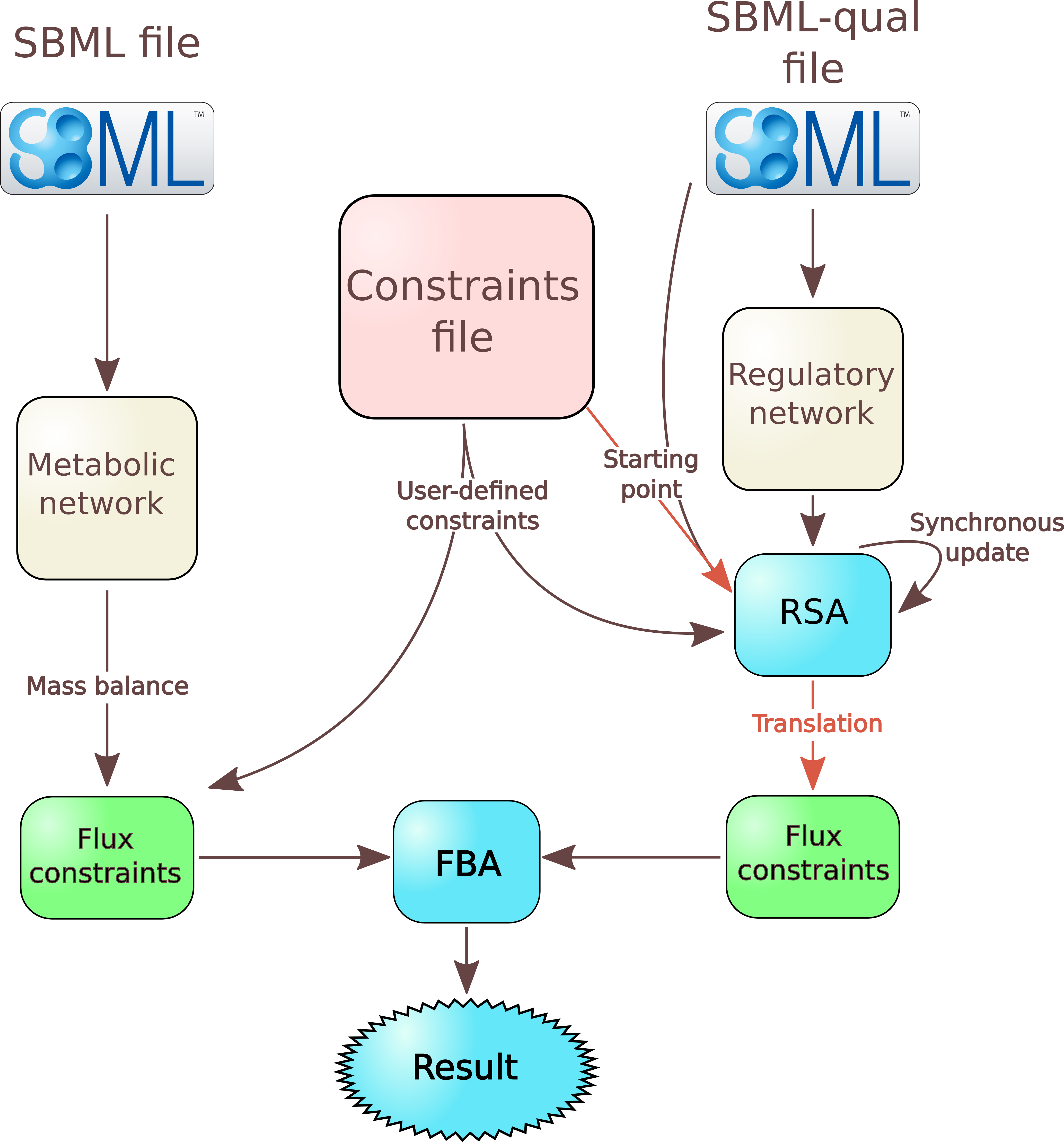
Concerning the regulatory network analysis, FlexFlux supports multistate qualitative regulatory networks. This regulatory network is composed of components of different natures (genes, mRNAs, proteins, metabolites ...), that interact with each other in different ways and can have an effect on the metabolic network. FlexFlux performs synchronous updates of the regulatory network state from provided initial values. Once a steady-state of this regulatory network is reached, the states are translated into continuous intervals (see the regulation file section) used as constraints for the FBA. We named this pipeline Regulatory Steady-state Analysis (RSA).
FlexFlux contains many methods dedicated to regulatory network and flux analysis. They are described below.
General functioning and file formats
FlexFlux works by taking as an input three different files:
- a file describing the metabolic network (SBML file format [ 1]),
- a constraint file containing the objective function as well as constraints concerning the values of variables,
- a regulation file describing the regulatory network in the SBML-qual [2] file format.
Overview of FlexFlux
File describing the metabolic network
From this file, FlexFlux performs a few actions:- it adds to the model all reactions, genes, and proteins as variables;
- consequently to the steady-state assumption, it adds constraints corresponding to the steady state;
- it adds all reaction flux constraints. If no value is given for a reaction, the lower bound is set to 0 for irreversible reactions and to -999999 for reversible ones, and the upper bound is set to 999999;
- it adds to the model all the logical constraints (as interactions) concerning gene-protein-reaction interactions (GPR).
Constraint file
The format of the constraint file is quite similar to existing file formats like the LP file format used by the solver CPLEX.
This file is used to define the objective function as well as constraints.
Objective function
To set the objective function :
obj : MAX(2*a + -1*b)where a and b are variables. The variables must be separated by a "+" sign and the coefficients can be any real number.
Nested objective functions
Multiple objective functions can be written. In that case, all objective functions are sequentially considered. The optimal value of an objective function becomes a new constraint (with a percentage of liberty than can be specified) for the following optimization.
Example :
obj : MAX(R_GLC)
obj : MAX(R_BIOMASS)
FlexFlux will first calculate the maximum value for R_GLC, will add it as a constraint, and then will normally continue with R_BIOMASS as the objective function
Constraints
Each line corresponds to a constraint :- The line may contain three columns :
a 3 6
which means 3 < a < 6 - Or two columns :
b -1
which means b=-1
By default, variables are considered as real numbers (they can take every value between their lower and upper bound, including decimal numbers).
If you don't want your variable to be a real number, you can set as a integer or a binary variable.
To add integer variables, they must be written under the line
INTEGERThe lines :
INTEGER

a 3 6
mean that a can take the value 3, 4, 5 or 6.
For binary values (0 or 1), the variable name has to be written under the line BINARY.
To set it to 0 or 1, the value must be written next to the variable. The lines :BINARY a b 1mean : a is a boolean and can be equal to 0 or 1 and b is a boolean equal to 1.
Starting points
In the constraint file, you can also specify starting points that will be used for the Regulatory Steady-state Analysis (RSA) (overview). They must be provided under the line :STARTING POINTExample :
STARTING POINT

allolactose	0
P_lacI	0
These starting points must be written after the other constraints but before the equations.
Equations
Equations can be added under the lineEQUATIONSThese equations must be composed of known variables and respect the following rules.
- Only one equality (or inequality) is possible by line. For example : 0 < a < 3*b will have to be written over two lines.
- Variables can be written without coefficient. If they have one, it must be placed before the variable name. Exemple 3*a + 4*b < 5.
- The negative sign must be on the coefficient : a+3*-b must be written : a + -3*b.
Equations can be a good way of making a shortcut, for instance :
obj : MAX(a)

.....

EQUATIONS
a = R_GLC + -2*R_AC + 3*R_BIOMASS
Example
Example of a constraint file :
obj : MAX(R_BIOMASS)

a 5
c 10
d 0 50
M_glc_D_b 10.4
M_ac_b 0.3

M_lcts_b 5.8

lacZ 0.001 0.03

R_EX_glc_e_ -10.5 999999
R_EX_o2_e_ -15 999999

R_EX_ac_e_ -2.5 4

R_EX_lcts_e_ -3 999999

INTEGER

BINARY

STARTING POINT

allolactose	0
P_lacI	0

EQUATIONS
d = 2*a + 3*c
Regulation file
This file corresponds to the description of a regulatory network with multi-state qualitative variables in the XML based SBML-qual file format.
As decribed in [2], components of the network must be added as qualitativeSpecies by specifying an initial qualitative value and the maximum number of states that this variable can have.
Updates
rules for each component are described in the Transition tags : each component has a default value and rules depending on other component states.
FlexFlux uses the given initial values and update rules to update the network state using synchronous update. Once a state that was already found is reached, an attractor has been found. FlexFlux then uses this attractor to create constraints used in the FBA.
FlexFlux allows to translate qualitative states into continuous intervals used as constraints for the FBA. The correspondance between qualitative state and coninutous interval must be specified by the user as a note in the qualitativeSpecies tag.
Example :<qual:qualitativeSpecies qual:id="A" qual:initialLevel="0" qual:maxLevel="2"> <notes> <body xmlns="http://www.w3.org/1999/"> <p>STATE 0:[0,1[</p> <p>STATE 1:]1,4.5]</p> <p>STATE 2:]4.5,+inf]</p> <p>STATE 3:ND</p> </body> </notes> </qual:qualitativeSpecies>ND means that this state corresponds to no constraint.
Key words
Getting the summation of all fluxes
The key-word FluxSum can be used to get the sum of the absolute values of all fluxes in the network.
It can be used for instance as an objective function :
obj : MIN(FluxSum)
It can be also used as a constraint :
FluxSum 0 3000
FlexFlux functions
This section details all possible analyses using FlexFlux. FlexFlux can used in two modes:
- Graphical version: GraphicalFlexflux.sh for linux and GraphicalFlexflux.bat for windows (see the installation section). Then choose your options and hit the run button!
- Command line. The arguments are the same. In this documentation, analyses are run in the command line but there is no difference.
To try the examples of this documentation yourself, you must change the name of the analysis acording to your operating system (see the installation section).
For example, for windowsFlexfluxFBA -s ....
becomesFlexflux.bat FBA -s ....
and for linux it becomes./Flexflux.sh FBA -s ....
The output of all analyses can be either a text file containing all the results data, a graphical representation of the data, or both.
Regulatory steady-state analysis : RSA
This function does not containt a FBA. Finds an attractor or the steady state of a given regulatory network with given initial values.Command-line arguments
- -reg String : Regulation file path
- -out String : [OPTIONAL]Output file name
- -cons String : [OPTIONAL]Constraint file path
- -plot : [OPTIONAL, default = false]Plots the results
Example :
FlexfluxRSA -reg regNetwork.xml -plot -out out.txt
Results
For this example, we search the attractor of a reconstructed regulatory model of the lac operon of E.Coli with both glucose and lactose available.We used :
- the regulation file lacOperon.sbml,
- the constraints file ConstraintsRSA.txt,
- the command line :
FlexfluxRSA -reg lacOperon.sbml -cons ConstraintsRSA.txt -out steady_states_result.txt -plot
Steady state analysis result

Entity name	State 1	State 2	State 3	State 4	State 5(Attractor)	Final constraint lower bound	Final constraint upper bound
EIIAGlc_p	0	0	0	0	0	0.0	0.0
lacI	1	1	1	1	1	1.0	1.0
M_lcts_b	3	3	3	3	3	5.8	5.8
M_glc_D_b	3	3	3	3	3	1.6	1.6
AMPc	0	1	1	1	1	1.0	1.0
permease	0	0	0	0	0	0.0	0.0
lacZ	0	1	0	1	1	1.0	1.0
CAP	1	1	1	1	1	1.0	1.0
lacY	0	1	0	1	1	1.0	1.0
P_lacI	0	1	0	0	0	0.0	0.0
R_LCTStpp	0	0	0	0	0	0.0	0.0
EIIAGlc	1	1	1	1	1	1.0	1.0
betaGal	0	0	1	0	1	1.0	1.0
R_LACZ	0	0	0	0	0	0.0	0.0
allolactose	0	1	1	1	1	1.0	1.0
The graphical result :
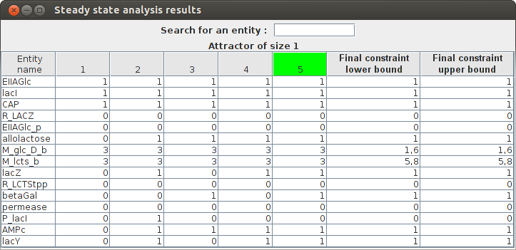
FlexFlux Regulatory steady-state analysis results. The state of the network is updated from the initial values given in the regulation file. The attractor found in shown in green (state 5 here).
This results shows that the steady-state found in this analysis corresponds to the utilisation of glucose by E.Coli and the repression of lactose utilisation.Simple FBA
Computes a simple FBA and returns the value of the optimized objective function as well as all variable values. Variable values can represent only one solution amongst many. The FBA can be constrained with calculated steady-states of a given regulatory network.Command-line arguments
- -s String : Sbml file path
- -cons String : Constraint file path
- -reg String : [OPTIONAL] Regulation file path
- -states : [OPTIONAL] The states of the regulatory network are saved in the indicated file name
- -out String : [OPTIONAL]Output file name
- -plot : [OPTIONAL, default = false]Plots the results
- -lib Double : [OPTIONAL, default = 0]Percentage of non optimality for new constraints
- -pre Integer : [OPTIONAL, default = 6]Number of decimals of precision for calculations and results
- -sol String : Solver name
- -ext : [OPTIONAL, default = false]Uses the extended SBML format
- -senFile : [OPTIONAL] A sensitivity analysis is performed and saved in the indicated file name
- -h : Prints help
Example :
FlexfluxFBA -s network.xml -cons cons.txt -reg regNetwork.xml -plot -out out.txt
Results
For this example, we use the FBA function to calculate all reaction fluxes of E.Coli metabolic network after the lac regulatory network steady state has been found.We used :
- the SBML file coli.xml,
- the constraint file constraintsFBA_coli.txt,
- the regulation file lacOperon.sbml,
- the command line :
FlexfluxFBA -s coli.xml -cons constraintsFBA_coli.txt -out FBA_result.txt -reg lacOperon.sbml -plot
FBA result

obj : 0.592258
b2309_and_b2307_and_b2306_and_b2308	Not Constrained
b4031	Not Constrained
b4032	Not Constrained
b4033	Not Constrained
b4034	Not Constrained
R_PANTS	3.41E-4
M_actp_c	Not Constrained
R_G6Ptex	0.0
R_12DGR141tipp	0.0
M_thex2eACP_c	Not Constrained
R_ASCBptspp	0.0
M_tym_p	Not Constrained
R_DXPRIi	0.001415
The graphical result :
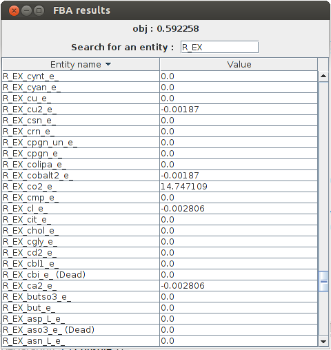
FlexFlux FBA results. In these conditions, given the constraints from the steady state of the regulatory network, the maximum biomass production is 0.592258 and we can see the value of all other variables.
In the output, we can see all the reaction fluxes corresponding to glucose utilisation by E.Coli. This particular phenotype is forced by the regulatory network steady state.Flux Variability Analyses : FVA
An FVA consists in getting the optimal value for the objective function, setting this value as a constraint and, given a list of entities, minimize and maximize their values. This analysis returns the objective value, and the minimum and maximum value for each entity desired.
The advantage of FlexFlux's FVA compared to classical FVA is that it is not limited to biochemical reactions. It can be done on any variable.
Command-line arguments
- -s String : Sbml file path
- -cons String : Constraint file path
- -reg String : [OPTIONAL]Regulation file path
- -e String : [OPTIONAL]Biological entities to perform the FVA on (Space-separated list of entities, example : "R1 R2 G1 G2"). If empty, FVA is done on all reactions
- -n Integer : [OPTIONAL, default = number of available processors]Number of threads
- -out String : [OPTIONAL]Output file name
- -plot : [OPTIONAL, default = false]Plots the results
- -lib Double : [OPTIONAL, default = 0]Percentage of non optimality for new constraints
- -pre Integer : [OPTIONAL, default = 6]Number of decimals of precision for calculations and results
- -sol String : Solver name
- -ext : [OPTIONAL, default = false]Uses the extended SBML format
- -h : Prints help
Example 1 :
FlexfluxFVA -s network.xml -cons cons.txt -reg regNetwork.xml -plot -out out.txtThis example is a simple FVA analysis on all reactions described in network.xml.
Example 2 :
FlexfluxFVA -s network.xml -cons cons.txt -reg regNetwork.xml -plot -out out.txt -e "R1 R2 G1 G2" -lib 10Here, the FVA will be run on the reactions R1 and R2 and on the genes G1 and G2 with a liberty of 10% for the objective constraint.
Results
For this example, we use the FVA function to calculate the minimal and maximal flux values of all E.Coli biochemical reactions when optimising its growth with no constraint.We used :
- the SBML file coli_core.xml,
- the constraint file constraintsFBA.txt,
- the command line :
FlexfluxFVA -s coli_core.xml -cons constraintsFBA.txt -out FVA_result.txt -lib 10 -plot
FVA result

obj : 0.873922(+-10.0%)
Name	min	max
R_CYTBD	35.984865	51.239087
R_PPCK	0.0	17.161
R_PGM	-16.732521	-8.686588
R_Biomass_Ecoli_core_w_GAM	0.786529	0.873922
R_SUCCt3	0.0	22.881333
R_PPC	0.0	20.346866
R_GLNabc	0.0	0.0
R_SUCOAS	-8.045934	0.0
R_CS	0.848587	8.89452
R_EX_glu_L_e	0.0	1.271185
R_EX_akg_e	0.0	1.430083
The graphical result :
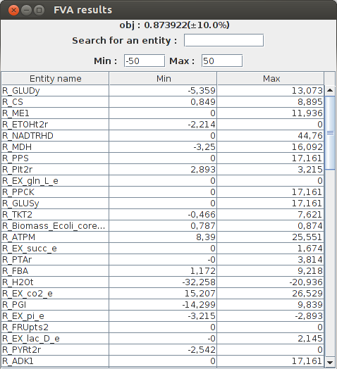
FlexFlux FVA results. Minimum and maximum flux of each reaction for a maximized biomass production (with a liberty of 10%).
Comparison of two FVAs
Compares the results of two FVA analyses given a metabolic network, an objective function and two different set of constraints. Constraints can be obtained with calculated steady-states of a given regulatory network. This analysis returns the objective value, the minimum and maximum value for each entity desired, for both conditions.Command-line arguments
- -s String : Sbml file path
- -cons String : Constraint file path
- -cons2 String : Second constraint file path
- -reg String : [OPTIONAL]Regulation file path
- -e String : [OPTIONAL]Biological entities to perform the FVA analyses on (Space-separated list of entities, example : "R1 R2 G1 G2"). If empty, FVA is done on all reactions
- -n Integer : [OPTIONAL, default = number of available processors]Number of threads
- -out String : [OPTIONAL]Output file name
- -plot : [OPTIONAL, default = false]Plots the results
- -lib Double : [OPTIONAL, default = 0]Percentage of non optimality for new constraints
- -pre Integer : [OPTIONAL, default = 6]Number of decimals of precision for calculations and results
- -sol String : Solver name
- -ext : [OPTIONAL, default = false]Uses the extended SBML format
- -h : Prints help
Example 1 :
FlexfluxCompFVA -s network.xml -cons cons.txt -cons2 cons2.txt -reg regNetwork.xml -plot -out out.txt
Example 2 :
FlexfluxCompFVA -s network.xml -cons cons.txt -cons2 cons2.txt -reg regNetwork.xml -plot -out out.txt -e "R1 R2 G1 G2"
Results
For this example, we use the FVA comparison function to compare minimal and maximal flux values of all E.Coli biochemical reactions when optimising its growth under two different conditions :- No constraint.
- Constrained glucose uptake.
We used :
- the SBML file coli_core.xml,
- the constraint file constraintsFBA.txt,
- a second constraint file constraintsFBA2.txt in witch we allow glucose uptake to be bigger,
- the command line
FlexfluxCompFVA -s coli_core.xml -cons constraintsFBA.txt -cons2 constraintsFBA2.txt -out comp_FVA_result.txt -lib 5 -plot
FVA comparison result

obj1 : 0.873922(+-5.0%)
obj2 : 1.790569(+-5.0%)
Name	min1	max1	min2	max2
R_EX_succ_e	0.0	0.837122	0.0	1.715171
R_ADK1	0.0	8.5805	0.0	17.5805
R_GLUSy	0.0	8.5805	0.0	17.5805
R_GLUDy	-4.950357	4.265735	-10.142737	8.740022
R_FORt2	0.0	34.322	0.0	70.322
R_FUM	0.792103	7.381819	1.021209	14.146736
R_EX_glc_e	-10.0	-9.523306	-20.0	-19.023306
R_PDH	3.903028	18.770887	6.937593	36.503884
R_GLUt2r	-0.635593	0.0	-1.302259	0.0
R_EX_o2_e	-23.709518	-19.895962	-45.644797	-37.831242
The graphical result :
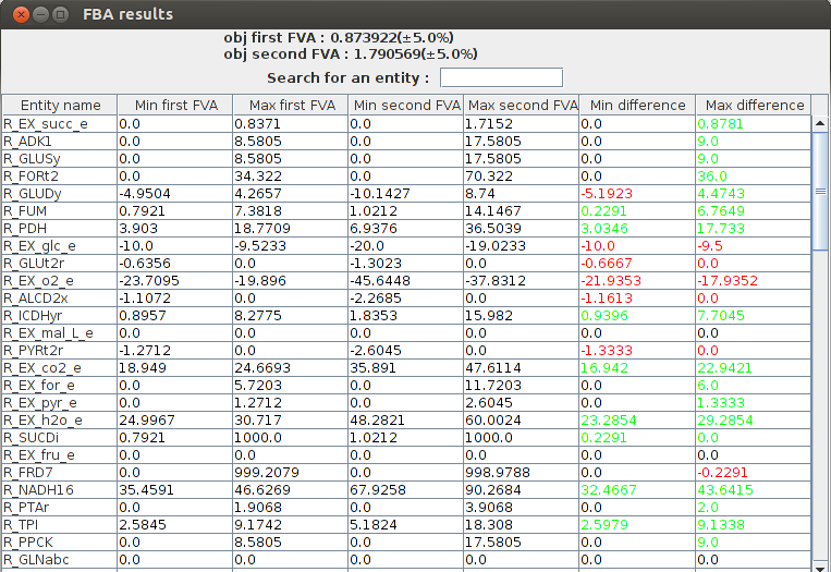
FlexFlux FVA comparison result. We can see the differences between the two conditions. The glucose uptake is bigger in the second case so the biomass production is higher. The two last columns make the comparison between the the FVA's easier. Green values mean the result is higher is the second condition, and red values mean the result is lower in the second condition.
Knock out analysis : KO
A KO analysis consists in setting network entities values to 0, and observe the effect on the objective function. There are three ways to perform this KO analysis:- on reactions,
- on genes,
- on any biological entity (specified with argument -e)
Command-line arguments
- -s String : Sbml file path
- -cons String : Constraint file path
- -reg String : [OPTIONAL]Regulation file path
- -e String : [Optional]Biological entities to perform the KO analysis on (Space-separated list of entities, example : "R1 R2 G1 G2"). If empty, KO is done on all reactions (mode 0) or all genes (mode 1)
- -mode Integer : [OPTIONAL, default = 0]KO mode :
- Mode 0: the KO analysis is performed on reactions.
- Mode 1: the KO analysis is performed on genes.
- -n Integer : [OPTIONAL, default = number of available processors]Number of threads
- -out String : [OPTIONAL]Output file name
- -plot : [OPTIONAL, default = false]Plots the results
- -lib Double : [OPTIONAL, default = 0]Percentage of non optimality for new constraints
- -pre Integer : [OPTIONAL, default = 6]Number of decimals of precision for calculations and results
- -sol String : Solver name
- -ext : [OPTIONAL, default = false]Uses the extended SBML format
- -h : Prints help
Example 1 :
FlexfluxKO -s network.xml -cons cons.txt -reg regNetwork.xml -plot -out out.txt -mode 1This example is a simple KO analysis run on all network genes (mode = 1).
Example 2 :
FlexfluxKO -s network.xml -cons cons.txt -reg regNetwork.xml -plot -out out.txt -e "R1 R2 G1 G2"Here the KO analysis is run on the reactions R1 and R2 and the genes G1 and G2.
Results
For this example, we use the KO function to see the effect of all individual genes KOs on the growth rate of E.Coli.We used :
- the SBML file coli_core.xml,
- the constraint file constraintsFBA.txt,
- the command line :
FlexfluxKO -s coli_core.xml -cons constraintsFBA.txt -out KO_result.txt -mode 1 -plot
KO results :

b2277 obj value : 0.211663
b1819 obj value : 0.873922
b3528 obj value : 0.873922
b2296 obj value : 0.873922
b3612 obj value : 0.873922
b2285 obj value : 0.211663
b0720 obj value : 0.0
b2914 obj value : 0.873922
The graphical result :
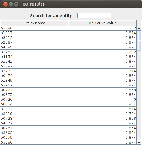
FlexFlux KO analysis result. The analysis is performed on genes because we set the parameter "mode" to 1. We can see what genes are essentials for biomass production. For exemple the gene b0720 is essential because the maximum biomass production is 0 when this gene is knocked out.
Time dependent FBA
This analysis is based on external metabolic concentrations and cell density. Given initial metabolite concentrations, cell density, a time step and a number of iterations, this analysis returns the value of each metabolite and cell density for each time. Initial metabolite concentrations must be written in the constraint file.
Command-line arguments
- -s String : Sbml file path
- -cons String : Constraint file path
- -reg String : [OPTIONAL]Regulation file path
- -e String : [OPTIONAL]Biological entities included in the results. If empty, only concerned metabolites and cell density will be included
- -x Double : Cell density initial value in g/L
- -t Double : [OPTIONAL, default = 0.1]Time between each iteration in hour
- -it Integer : [OPTIONAL, default = 150]Number of iterations
- -bio String : Name of the biomass reaction
- -out String : [OPTIONAL]Output file name
- -plot : [OPTIONAL, default = false]Plots the results
- -lib Double : [OPTIONAL, default = 0]Percentage of non optimality for new constraints
- -pre Integer : [OPTIONAL, default = 6]Number of decimals of precision for calculations and results
- -sol String : Solver name
- -ext : [OPTIONAL, default = false]Uses the extended SBML format
- -h : Prints help
Example 1:
FlexfluxTDRFBA -s network.xml -cons cons.txt -reg regNetwork.xml -bio R_BIOMASS -x 0.01 -plot -out out.txtThis a a RFBA analysis on the network described in network.xml. The biomass reaction is R_BIOMASS and the initial cell density is 0.01 g/L.
Example 2:
FlexfluxTDRFBA -s network.xml -cons cons.txt -reg regNetwork.xml -bio R_BIOMASS -plot -out out.txt -x 0.01 -t 0.02 -it 400 -e "R1 R2 G1 G2"Here, the timestep between each iteration will be 0.02 h and the entities R1, R2, G1 and G2 will be added to the results.
Results
For this example, we use the Time dependent FBA function to follow diauxic growth of E.Coli on gluocose and lactose over 15 hours.We used :
- the SBML file coli.xml,
- the constraint file constraintsFBA_coli.txt where initial concentrations are set,
- the regulation file lacOperon.sbml,
- The command line:
FlexfluxTDRFBA -s coli.xml -cons constraintsFBA_coli.txt -reg lacOperon.sbml -out TDRFBA_result.txt -bio R_BIOMASS -e lacZ -x 0.011 -plot
The values for this example are extracted from [3] and algorithms for calculations are detailed in [6].
Here is a part of the text result file TDRFBA_result.txt :Time M_lcts_b lacZ X M_glc_D_b 0.0 5.8 0.0 0.011 1.6 0.1 5.8 0.0 0.011671 1.592634 0.2 5.8 1.0 0.012383 1.584819 0.3 5.8 1.0 0.013139 1.576526 0.4 5.8 1.0 0.013941 1.567728 0.5 5.8 1.0 0.014791 1.558393 0.6 5.8 1.0 0.015694 1.548488 0.7 5.8 1.0 0.016651 1.53798 0.8 5.8 1.0 0.017667 1.526829 0.9 5.8 1.0 0.018745 1.514999 1.0 5.8 1.0 0.019889 1.502447
The graphical result :
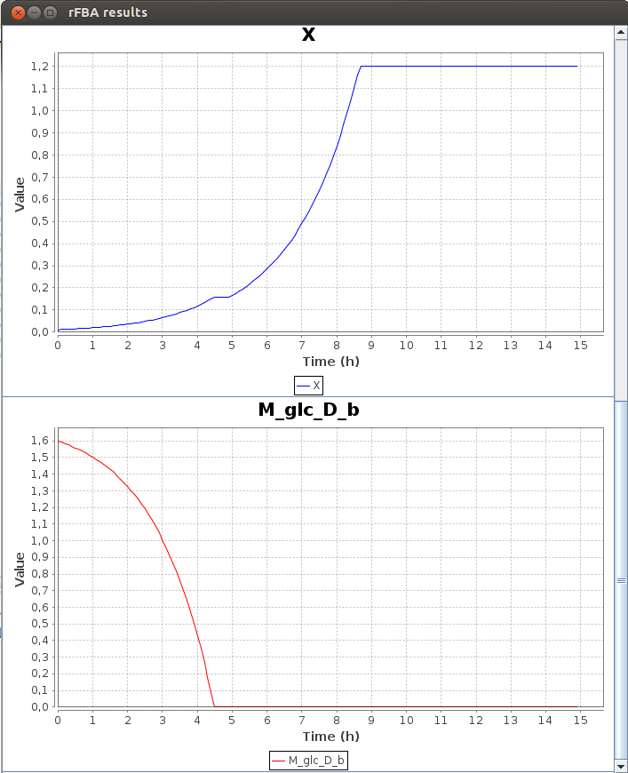
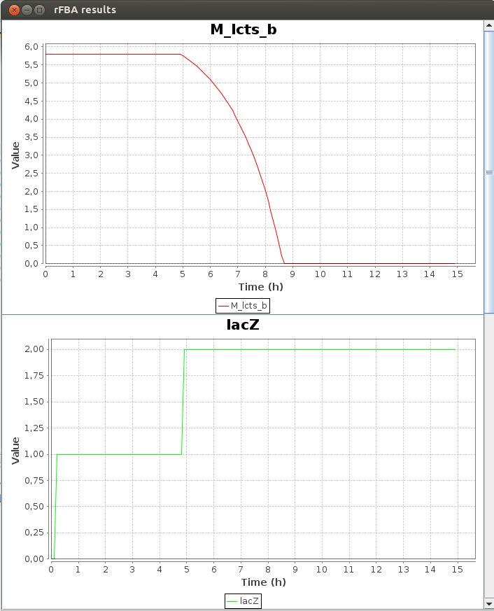
FlexFlux time dependant flux analysis result. We can see the variation of the value of differents entities. X represents the cell density. While the glucose concentration (M_glc_D_b) is greater than 0, the gene lacZ is not activated. When all the glucose is used, lacZ is activated and the cell can use the lactose to grow.
We can see that the lac regulatory network of E.Coli force utilisation of glucose first, and then when it runs out, switches to lactose utilisation, with a lower growth rate.2-D Phenotypic phase analysis
This analysis returns the objective value for each reaction flux.
This permits a phenotype phase plane analysis. [4]
A phenotype phase corresponds to a specific metabolic network behavior.
In order to do that, it calculates the shadow price on each point and groups the points with same shadow price into phenotipic phases that are represented in different colors. To give a hint on what reactions are active in each phase, a FVA is applied on each one and the result is graphically shown: essential reactions are displayed.
Command-line arguments
- -s String : Sbml file path
- -cons String : Constraint file path
- -reg String : [OPTIONAL]Regulation file path
- -r String : Name of the reaction to test
- -init Double : Initial flux value of the reaction to test
- -end Double : Final flux value of the reaction to test
- -f Double : [OPTIONAL, default = 0.1]Difference between each FBA for the reaction flux
- -n Integer : [OPTIONAL, default = number of available processors]Number of threads
- -out String : [OPTIONAL]Output file name
- -plot : [OPTIONAL, default = false]Plots the results
- -lib Double : [OPTIONAL, default = 0]Percentage of non optimality for new constraints
- -pre Integer : [OPTIONAL, default = 6]Number of decimals of precision for calculations and results
- -sol String : Solver name
- -ext : [OPTIONAL, default = false]Uses the extended SBML format
- -h : Prints help
Example :
FlexfluxPP2D -s network.xml -cons cons.txt -reg regNetwork.xml -r R1 -init -10 -end 0 -plot -out out.txt
Results
For this example, we use the 2-D Phenotypic phase analysis function to see the differents metabolic network behaviours of E.Coli depending on the value of oxygen uptake.We used :
- the SBML file coli_core.xml,
- the constraint file constraintsFBA.txt,
- the command line :
FlexfluxPP2D -s coli_core.xml -cons constraintsFBA.txt -out PP2D_result.txt -r R_EX_o2_e -init -20 -end 0 -f 0.05 -plot
Reaction flux result

Flux : R_EX_o2_e
Objective : R_Biomass_Ecoli_core_w_GAM

Flux	Objective
-20.0	0.832614
-19.95	0.831466
-19.9	0.830318
-19.85	0.82917
-19.8	0.828023
-19.7	0.825727
-19.75	0.826875
The graphical result :
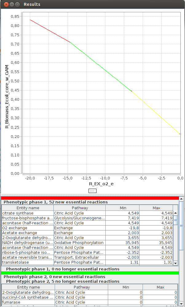
FlexFlux 2-D Phenotypic phase analysis. We can see the evolution of the maximum biomass production for different values of oxygen uptake.
We can observe three distinctive phenotypic phases. This shows that E.Coli can respond in three different ways to oxygen concentrations.3-D Phenotypic phase analysis
This analysis returns the objective value for each combination of two reaction fluxes.
This permits a phenotype phase plane analysis.
In order to do that, it calculates the shadow price on each point and groups the points with same shadow price into phetotipic phases that are represented in different colors. To give a hint on what reactions are active in each phase, a FVA is applied on each and the result is graphically shown : essential reactions are displayed (the "order" found for the phases is only indicative and might not have any biological meaning).
Command-line arguments
- -s String : Sbml file path
- -cons String : Constraint file path
- -reg String : [OPTIONAL]Regulation file path
- -r String : Name of the first reaction to test
- -r2 String : Name of the second reaction to test
- -init Double : Initial flux value of the first reaction to test
- -end Double : Final flux value of the first reaction to test
- -f Double : [OPTIONAL, default = 0.1]Difference between each FBA for the first reaction flux
- -init2 Double : Initial flux value of the second reaction to test
- -end2 Double : Final flux value of the second reaction to test
- -f2 Double : [OPTIONAL, default = 0.1]Difference between each FBA for the second reaction flux
- -n Integer : [OPTIONAL, default = number of available processors]Number of threads
- -out String : [OPTIONAL]Output file name
- -plot : [OPTIONAL, default = false]Plots the results
- -lib Double : [OPTIONAL, default = 0]Percentage of non optimality for new constraints
- -pre Integer : [OPTIONAL, default = 6]Number of decimals of precision for calculations and results
- -sol String : Solver name
- -ext : [OPTIONAL, default = false]Uses the extended SBML format
- -h : Prints help
Example:
FlexfluxPP3D -s network.xml -cons cons.txt -reg regNetwork.xml -r R1 -init -20 -end 0 -r2 R2 -20 -end2 0 -f2 0.2 -plot -out out.txt
Results
For this example, we use the 3-D Phenotypic phase analysis function to see the differents metabolic network behaviours of E.Coli depending on the value of oxygen and glucose uptake.We used :
- The SBML file coli_core.xml
- The constraint file constraintsFBA.txt
- The command line :
FlexfluxPP3D -s coli_core.xml -cons constraintsFBA.txt -out PP3D_result.txt -r R_EX_glc_e -init -20 -end 0 -f 0.5 -r2 R_EX_o2_e -init2 -20 -end2 0 -f2 0.05 -plot
Two reactions fluxes result

Flux1 : R_EX_glc_e
Flux2 : R_EX_o2_e
Objective : R_Biomass_Ecoli_core_w_GAM

Flux1	Flux2	Objective
-20.0	-19.5	1.192735
-20.0	-20.0	1.208983
-20.0	-19.0	1.176487
-20.0	-18.5	1.160239
-20.0	-17.5	1.127742
-20.0	-18.0	1.14399
-20.0	-16.5	1.095245
-20.0	-16.0	1.078997
-20.0	-15.5	1.062749
-20.0	-17.0	1.111494
-20.0	-15.0	1.0465
The graphical result :
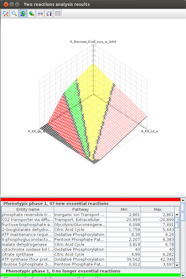
FlexFlux 3-D Phenotypic phase analysis result. We can see the evolution of the maximum biomass production for different values of oxygen and glucose uptake. We observe four distinctive phenotypic phases.
Pareto analysis
The goal of this analysis is to determine what objective (or set of objectives) an organism is optimizing.[5]
It take as an argument a file containing the objective functions to test and experimental values, and finds out (in one, two and three dimensions) what objective optimization is closest to the experimental values.
The objectives that are optimized are those for witch the experimental values are the closest to the pareto surface.
The pareto surface is the surface in which all points are pareto optimal. This means that to increase the value of an objective, you must decrease another.
In this analysis, the objective function of the constraints file is optional and ignored if present.
Objective function and experimental values file
The file must contain all the objectives in the first line, and then one line per experimental value. There must be as many values for one experiment as there are objective functions.
For each experimental value, values for the objectives must be in order and separated by a space.
Example:
MIN(sum) MAX(atpYield) MAX(R_Biomass_Ecoli_core_w_GAM)

1667.4 213.0 6.4
1635.9 191.0 7.9
1622.2 204.0 7.2
1640.4 171.0 7.4
1696.2 176.0 7.2
1657.4 173.0 7.4
1642.9 207.0 6.9
1616.7 185.0 7.7
1569.8 198.0 7.8
Command-line arguments
- -s String : Sbml file path
- -cons String : Constraint file path
- -reg String : [OPTIONAL]Regulation file path
- -exp String : Path of file containing objective functions and experimental values
- -all : [OPTIONAL, default = false]Plots all results. If false, plots 1D results and only the best result for 2D and 3D results.
- -n Integer : [OPTIONAL, default = number of available processors]Number of threads
- -out String : [OPTIONAL]Output folder name
- -plot : [OPTIONAL, default = false]Plots the results
- -lib Double : [OPTIONAL, default = 0]Percentage of non optimality for new constraints
- -pre Integer : [OPTIONAL, default = 6]Number of decimals of precision for calculations and results
- -sol String : Solver name
- -ext : [OPTIONAL, default = false]Uses the extended SBML format
- -h : Prints help
Example : FlexfluxPareto -s network.xml -cons cons.txt -int regNetwork.xml -plot -e expFile
Results
For this example, we used :- the SBML file coli_core.xml
- the constraint file constraintsPareto.txt
- the objective/experimental file expFile.txt
- the command line:
FlexfluxPareto -s coli_core.xml -cons constraintsPareto.txt -exp expFile.txt -out pareto/ -plot
The graphical results :
Axes values are normalized such that the coordinates of the points on the Pareto surface range from 0 to 1, where 1 represents the theoretical minimum or maximum of an objective.
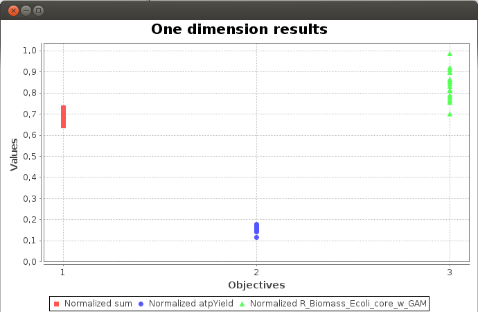
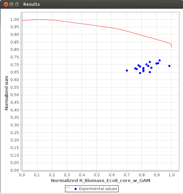
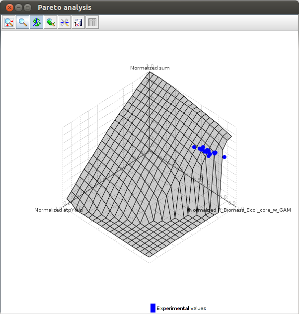
FlexFlux Pareto analysis result.
Dead reactions
Dead reactions are unable to carry a steady state flux and thus clearly represent missing information in the model. This analysis returns the list of dead reactions.Command-line arguments
- -s String : Sbml file path
- -cons String : [OPTIONAL]Constraint file path
- -reg String : [OPTIONAL]Regulation file path
- -d Double : [OPTIONAL, default = 0.000001]Maximal distance of the reaction flux from 0 to be considered as dead
- -mode Integer : [OPTIONAL, default = 0]Dead reactions mode:
- - Mode 0: Reactions fluxes are not changed.
- - Mode 1: All reactions fluxes bounds are set to a maximum value. (fluxes become free)
- -n Integer : [OPTIONAL, default = number of available processors]Number of threads
- -out String : [OPTIONAL]Output file name
- -plot : [OPTIONAL, default = false]Plots the results
- -lib Double : [OPTIONAL, default = 0]Percentage of non optimality for new constraints
- -pre Integer : [OPTIONAL, default = 6]Number of decimals of precision for calculations and results
- -sol String : Solver name
- -ext : [OPTIONAL, default = false]Uses the extended SBML format
- -h : Prints help
Example 1 : FlexfluxDR -s network.xml -plot -out out.txt
Example 2 : FlexfluxDR -s network.xml -cons cons.txt -reg regNetwork.xml -plot -out out.txt -mode 1 -d 0.1
Results
For this example, we used :- the SBML file coli_core.xml,
- the command line :
FlexfluxDR -s coli_core.xml -out DR_result.txt -plot
Dead Reactions result

R_EX_fru_e
R_EX_fum_e
R_EX_mal_L_e
R_FUMt2_2
R_GLNabc
R_EX_gln_L_e
R_FRUpts2
R_MALt2_2
The graphical result :
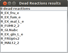
FlexFlux dead reaction identification result. In these conditions, those 8 reactions cannot carry any flux
Biological Entity Clustering by their contribution to the Objective Function (BECO)
The BECO method has been designed to classify the biological entities (reactions, genes, regulators) depending on their contribution to several objectives in several conditions and to cluster the objective functions and the conditions depending on the optimal values of each objective function in each condition.Command-line arguments
Input data files
- -s String: Path to the Sbml or MetExploreXml file containing the metabolic network
- -ext: [OPTIONAL, default = false] Uses the MetExploreXml format instead of SBML format for the metabolic network
- -cons String: [OPTIONAL] Constraint file
- -reg String: [OPTIONAL] Path to the regulation file path (SBML-QUAL format)
- -cond String : File describing conditions (set of initial states)
- -o String: Path to the file containing the objective functions
- -out: [OPTIONAL] Path to the output file directory
Parameters for biological entity clustering
- -inchlibPath: Path to the inchlib program [default=/usr/local/inchlib_clust/inchlib_clust.py]
- -mdg: [OPTIONAL] Gene metadata file used for heatmap analysis
- -mdr: [OPTIONAL] Reaction metadata file used for heatmap analysis
- -mdreg File: [OPTIONAL] Regulator metadata file used for heatmap analysis
- -mdSep String: [Default=,] Separator for the columns in the metaData file
- -noGeneAnalysis: Don't perform gene clustering
- -noReactionAnalysis: Don't perform reaction clustering
- -noRegulatorAnalysis: Don't perform regulator clustering
- -fixConditions: [OPTIONAL] If true, the conditions set in the condition file are fixed and can not be updated by the regulation network
Other parameters
- -cytoscape: [OPTIONAL]Generates cytoscape files representing reaction classification for each pair condition/objective
- -plot: [OPTIONAL, default = false] Plots the condition/objective heatmap
- -lib Double: [OPTIONAL, default = 0] Percentage of non optimality for new constraints
- -n Integer: [OPTIONAL, default = number of available processors] Number of threads
- -pre Integer: [OPTIONAL, default = 6] Number of decimals of precision for calculations and results
- -sol Solver: Solver name
- -verbose: [default=false] Activates the verbose mode
- -h: Prints this help
Overview
BECO performs several actions:- Condition and objective clustering
- Reaction clustering
- Metabolic gene clustering
- Regulator clustering
- Metabolic pathway clustering
Results
Condition and objective clustering
For each pair condition/objective, a FBA is performed. The conditions and the objectives are clustered considering the FBA results. In the root of the output directory, a file resultFBA.tab is generated. Each column j corresponds to an objective and each row i corresponds to a condition. Each cell (i,j) corresponds to the value of the objective function (j) considering the condition (i).Reaction clustering
For each pair condition/objective, a classification of the reactions depending of their contribution to the objective function is performed. The reactions and the pairs condition/objective are clustered considering the classication of the reactions. Reactions are classified into six classes inspired by Lewis et al. 2010:- Essential reactions
- Zero flux reactions
- Metabolically less efficient (MLE) reactions: enabling not optimal objective flux
- Enzymatically Less Efficient (ELE) reactions: enabling optimal flux but not the minimisation of the flux sum
- Objective Independant Reactions: reactions without effect on the objective function
- pFBA optima reactions: enabling optimal flux an also the minimisation of the flux sum
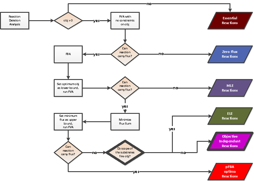
Reaction classification
Metabolic gene clustering
For each pair condition/objective, a classification of the metabolic genes depending of their contribution to the objective function is performed. The genes and the pairs condition/objective are clustered considering the classication of the genes.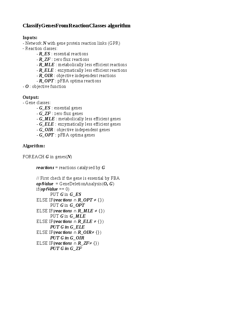
Gene classification algorithm
Regulator clustering
For each pair condition/objective, a classification of the actors of the regulatory network depending of their contribution to the objective function is performed. Regulators are classified into 3 categories:- Essential: if the regulator is inhibited, the optimal value of the objective function is null
- Optimal: if the regulator is inhibited, the optimal value of the objective function is decreased
- Neutral: if the regulator is inhibited, the optimal value of the objective function remains the same
References
-
Hucka M, Finney A, Sauro HM, Bolouri H, Doyle JC, Kitano H, Arkin AP, Bornstein BJ, Bray D, Cornish-Bowden A, Cuellar AA, Dronov S, Gilles ED, Ginkel M, Gor V, Goryanin II, Hedley WJ, Hodgman TC, Hofmeyr JH, Hunter PJ, Juty NS, Kasberger JL, Kremling A, Kummer U, Le Novère N, Loew LM, Lucio D, Mendes P, Minch E, Mjolsness ED, Nakayama Y, Nelson MR, Nielsen PF, Sakurada T, Schaff JC, Shapiro BE, Shimizu TS, Spence HD, Stelling J, Takahashi K, Tomita M, Wagner J, Wang J: The systems biology markup language (SBML): a medium for representation and exchange of biochemical network models. Bioinformatics 2003
-
Chaouiya C, Bérenguier D, Keating SM, Naldi A, van Iersel MP, Rodriguez N, Dräger A, Büchel F, Cokelaer T, Kowal B, Wicks B, Gonçalves E, Dorier J, Page M, Monteiro PT, von Kamp A, Xenarios I, de Jong H, Hucka M, Klamt S, Thieffry D, Le Novère N, Saez-Rodriguez J, Helikar T: SBML qualitative models: a model representation format and infrastructure to foster interactions between qualitative modelling formalisms and tools. BMC Syst Biol 2013
-
Markus W. Covert and Bernhard Ø. Palsson: Transcriptional Regulation in Constraints-based Metabolic Models of Escherichia coli.The Journal of Biological Chemistry 2002
-
Jeremy S. Edwards, Ramprasad Ramakrishna, Bernhard O. Palsson: Characterizing the Metabolic Phenotype: A Phenotype Phase Plane Analysis. Biotechnology and bioengineering 2002
-
Robert Schuetz, Nicola Zamboni, Mattia Zampieri, Matthias Heinemann, Uwe Sauer: Multidimensional Optimality of Microbial Metabolism. Science 2012
-
Amit Warma and Bernhard Ø Palsson: Stoichiometric flux balance models quantitatively predict growth and metabolic by-product secretion in wild-type Escherichia coli W3110. Appl Environ Microbiol. 1994
-
Lewis NE, Hixson KK, Conrad TM, Lerman JA, Charusanti P, Polpitiya AD, et al. Omic data from evolved E. coli are consistent with computed optimal growth from genome-scale models. Mol Syst Biol. 2010 Jul;6:390.